In this other post, I explained that the local value of a commodity can be expressed in terms of c + v + s, where c is constant capital, v is variable capital, and s is surplus value. The value is the average of all local values of all firms, which is the value of the commodity that prices fluctuate around.
How, in practice, does one actually calculate the value of a commodity? You can think of all industries in a capitalist economy as a black box that takes in some inputs from other firms, constant capital, transforms those inputs into something new by applying human labor to it, and then sells those commodities in a new form. The labor here adds value to the commodity.
It is also important to recall that v + s are both derived from labor added. Therefore, we will refer to both of these together as a single unit, L, such that L = v + s. As a commodity moves up the supply chain, its value increases as at every level, firms purchase the commodity, apply labor to it which increases its value, and then sell it to the next firm at that value.

In order to calculate the full value of a commodity, we would need to know its entire supply chain. This would require something known as an input-output table. An input-output table represents all the inputs all firms in the economy takes and what firms it outputs all its commodities to. Below is an example of a simple input-output table for a simple economy that only produces bread and oil.
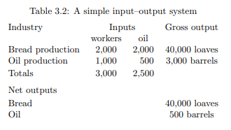
Let’s assume that this table represents a time scale of a single week. That is to say, in one week, 500 barrels of oil and 40,000 loaves of bread are produced. The constant value we need to find is labor time. Since this is a weekly time-scale, the number of workers will represent a constant value of 1 week. For the bread firm, it added 2,000 weeks of labor time per week to production of bread.
This can be solved by representing the whole system as a system of equations where each commodity is a variable while labor time is a constant. If we refer to bread as x and oil as y then we get this system of equations:

This one would be rather simple to solve. The second equation is fairly trivial to find the solution for by solving for by, resulting in y = 2/5, telling us that the value of a barrel of oil here is 0.4 weeks of labor, or 2.8 days worth of labor time. The second can now be solved by first solving for into x = (1+1y)/20 and simply by plugging in y. This will result in x = 0.07 or, in other words, the value of a single loaf of bread is 0.07 weeks of labor, or about 11.76 hours.
For a more complex input-output table, Gaussian elimination can be used. If you have never learned this, I highly recommend this video. In it, the author explains how to do the Gaussian elimination on a system of equations by hand. However, when planning an economy, we will not want to do things by hand, but by computer. So we will need to write up some algorithms to deal with this.
Let’s take the simple economy and add one more firm. This firm will be producing cars in order to do so, it requires both bread and oil. Of course, this might not make much sense, but let’s just go with it for simplicity.

This is similar to the other table provided above but with a cars row added and some other values changed. I also needed to add a column for bread now since some industries take bread as an input, and even though nothing takes cars as inputs, I added a cars column anyways. Notice how the rows are in the same order as the columns, with oil, bread, then cars. This often how input-output tables will be provided.
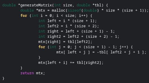
Here I will represent my input-output table as an array in C. I prefer to represent arrays, no matter how many dimensions, in a single dimension. It just keeps data easier to work with. Throughout this, I will use the variable “size” quite often. It just refers to the number of rows, in this case 3.

We will also want a function that could display the data in the table.


This matrix here is not the kind of matrix we need for Gaussian elimination. Some changes have to be made. In order to demonstrate what I mean, let’s convert it to a system of equations first.

Notice how the constants are on the left-hand-side while there are variables on the right-hand-side. The matrix needed for Gaussian elimination requires that the constants be on the right-hand-side by themselves and the variables all on the left-hand-side. The algorithm for this is quite simple, simply subtract the variables on the left-hand-side from the ones on the right-hand-side and this will isolate the constants.

This matrix now is arranged in a way that Gaussian elimination can be performed, with worker’s labor on the most right-hand column and the rest of the columns representing the inputs and outputs. Notice how some are negatives now. All columns, except for the last, now represent the gross output. Each row represents a different industry. A negative sign would mean that it consumes more of that commodity than it outputs. Such as, the car industry (third row) produces 50 cars, but consumes 1500 barrels of oil and 1000 loaves of bread.
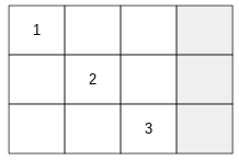
This matrix is now ready to have Gaussian elimination performed on it. The first step is to convert the matrix to Row Echelon form. You want to move through the elements in the array in the order shown below.
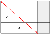
The last column is ignored in Gaussian elimination. Imagine a diagonal line going through the rest of the matrix. Each element below the diagonal line needs to be converted into a zero. The order we move through the matrix is the order I show. We start on the first column and last row, then we move up the rows, then when we’ve converted all those elements to zero, we then move onto the next column.
To convert an element to zero you need to perform an elementary row operation. An elementary row operation adds one row to another, multiplied by a factor. All we have to do is look for a row which we can multiply by a factor and then add to our current row to change the element to a zero. Here is some example code for an elementary row operation.

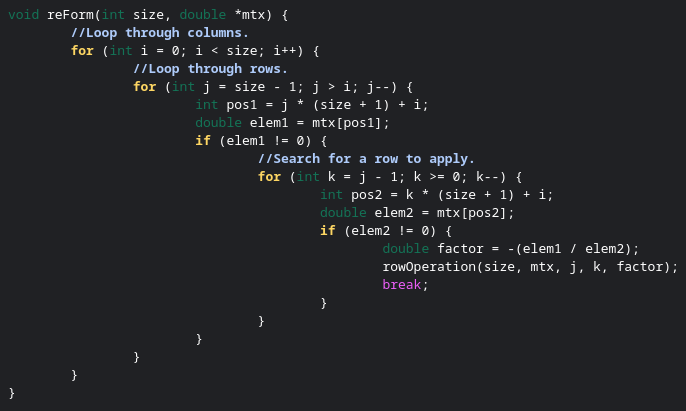
When look for a row that an elementary row operation can be applied to convert the element to a zero, we only have to check rows above the element in question. Why? Because the elements all below it have already been converted to zeros, and there is no elementary row operation that could be applied to convert the element to a zero if the row in question has a zero in the same column as the element. Below is an example of a function to convert a matrix to row echelon form.

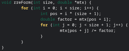
The final thing we need to do is convert this to reduced row echelon form. This is rather trivial. For each element on the diagonal, divide the entire row by the value on the diagonal. This will convert every element on the diagonal to a one.

Notice the last row. Whenever the algorithm finishes, the last row will tell us exactly the value of the last commodity. In this case, the value of a barrel of oil is 2 weeks of labor, the value of a loaf of bread is 0.15 weeks of labor, and the value of a car 163 weeks of labor.
In this case, we’re lucky. Notice how above the diagonal, all elements are zero. This isn’t always the case. Here is some modified data. When we run the Gaussian elimination, we do not get output as simple of an output as last time.


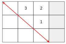
Notice how with the output here, the values above the diagonals are not zeros. It is relatively trivial to fix this, however. Simply step through the elements in the order shown below, and for each element, do an elementary row operation. The row you want to do the operation on is the same row as the column of the element, and the factor is the negative value of the element.
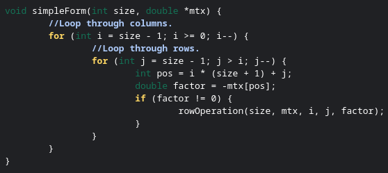

And there we go! The final column again gives us the values in term of labor time per week of every commodity in this simple economy. If we want, we can change the data to the simpler two-commodity economy we started with and see that this works.


As we can see, this matches our data prior. The values are always listed as the final column for every commodity. This method is by no means the fastest way of doing this, but it is simply meant to show how it can be done. Gaussian elimination can be parallelized (see here), making it fairly easy to scale.
This is by no means the fastest method. This method, however, is the easiest. This is a rather trivial algorithm that most university students will learn in school. There are other algorithms which can approximate values as well for producing approximate plans for large economies with fairly little computing power.
Note that if you have a much larger economy, many firms will be producing the same commodity. Some more notation will need to be added to the table to label firms that produce the same commodities. These firms will then need to have their local values averaged to get the final values. Or, on the other hand, if those collecting the data group together similar commodities beforehand, then the average will not need to be taken.


